A Junior Quant's Guide to Statistical Arbitrage [Code Included]

The hardest way to make an easy living...

Not too long ago, we began modeling and replicating some of the cash-cow strategies deployed by major quantitative hedge funds. So far, we’ve tightened a headlock on trend-following and momentum strategies, going as far as re-factoring them into a proprietary (and working) short vol strategy.

However, there’s one more, major cash cow we haven’t explored yet.

The big 3 strategies deployed by quant shops are trend following, momentum, and you guessed it… statistical arbitrage.

So, we’ll be venturing into these waters to find out exactly how it works, why it works, and exactly how much money it can make. As you’ll see shortly, successful stat arb is a lot more involved than just trading Pepsi and Coca-Cola.

Without spending another second, let’s get right into it.

WTH Is Stat Arb Anyway?

At its core, statistical arbitrage (stat arb) is a mean-reversion strategy that profits when one asset becomes over -or-under valued compared to another, similar asset. Now, even for companies that are nearly identical, there’ll always be differences in the prices you pay. Stat arb comes in when this divergence of prices becomes too far from the average. The strategy simply bets that over time, this divergence will decrease back to normal levels.

However, in order for the strategy to work, it is essential that we first make sure that the relationship between the assets are truly mean-reverting in the first place. To do this, we’ll go with the industry-standard Engle-Granger two-step method.

Assume we have 2 stocks we want to test, Stock A and Stock B.

First, we run a simple regression model that uses the price of Stock A to predict the price of Stock B. In theory, if the prices of these stocks truly moved together, then a regression model should be able to accurately predict the stock price with minimal errors.

Once the regression model is run, we then pull all of the errors the model made. For instance, if the model predicted stock B’s to be up 2%, but the real value was 1%, the error (the residual) is 1. When looking at the residuals, if we find that they tend to be around a certain mean with relatively stable variance, we can classify these residuals as stationary. A stationary time-series essentially means that data points tend to fluctuate right around the mean and tend to revert when they experience a divergence — exactly what we need.

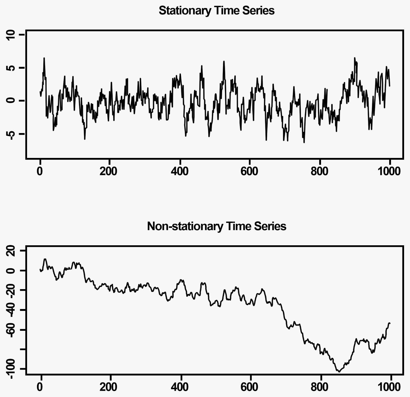
As a stat arb trader, your profits come from trading stationary relationships when the divergence becomes out of whack and reverts back to the mean. If the time series is non-stationary (see second sub-graph), you take losses as you await a reversion that never comes.

We test for this stationarity by running an Augmented Dickey-Fuller (ADF) test which returns a p-value letting us know whether the series is stationary or not. Our desired p-value of less than 0.05 essentially translates to “there is a 5% chance that this relationship is spurious (random) and non mean-reverting”.

Once we’ve run our tests and found a suitable pair, we can then move onto making actual trades.

How The Money Is Made

To begin, let’s take 2 closely related stocks; Ametek, Inc (NYSE: AME) and Dover Corp (NYSE: DOV). Both companies provide industrial electronic equipment, have overlapping market share, and are similarly priced:

Visually, you can see that when one over/underperforms relative to the other, that spread tends to shrink back down in the future. Here’s a visual representation of that spread:

After running an ADF Test on these returns, we learn that the P-Value is ~0.01 which confirms that the mean-reverting nature of the spread is statistically significant. Remember, the spread doesn’t need to have an average of 0 (identical returns), it just needs to have an average, say 10%, that the series normally reverts to.

Okay, so we know that the pair is both fundamentally linked and more importantly, stationary, but how do we know when to make a trade?

One school of thought is to use a fixed value, say; “initiate a trade when the spread is above 20”. The problem with this is that we would choose that value based on look-ahead bias — we only know that 20 is the usual limit by looking directly at those past observations from the future. Additionally, if we wanted to apply this strategy to a different pair, that fixed value may not be applicable.

Alternatively, we can go with an approach that initiate trades when the spread increases n-deviations above a rolling window. For example, “if the spread increases by more than 1 standard deviation above the 200-day average, we initiate a trade.”

Here’s what that would look like: