Sport Markets Aren't So Efficient After All... [Code Included]
From Finance to Sports, pulling money out of markets is only getting easier.
An efficient market is defined as a market where prices reflect all available information and there exist no room for excess profit or arbitrage. This is weakly seen in traditional Finance markets, most notably through the Efficient Market Hypothesis, but as we’ve repeatedly demonstrated, with a bit of creativity and work, profitable edges can be squeezed out of these markets.
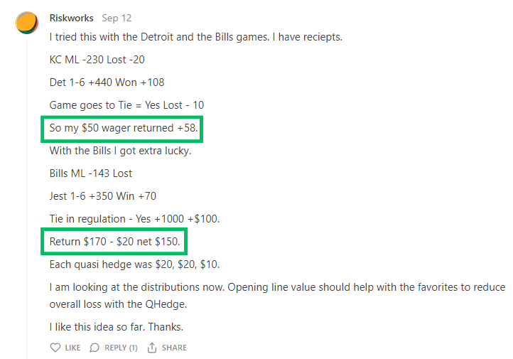
We’ve already begun to tear apart at the idea of efficient sport markets with our recent post on Quasi-Arbitraging, where a few readers have already profitably deployed the methods first-hand:
Much like in Finance, when a market is inefficient, we can get paid for making them efficient. So, before we re-visit and expand on what we can squeeze out risk-free, let’s put a system in place to get paid for stepping in when markets are wonky.
But before we dive-in, there’s a bit of background knowledge to cover.
Inefficient Markets: NFL Receptions
In the NFL, a reception is defined as when a player successfully catches the ball thrown by their own quarterback:
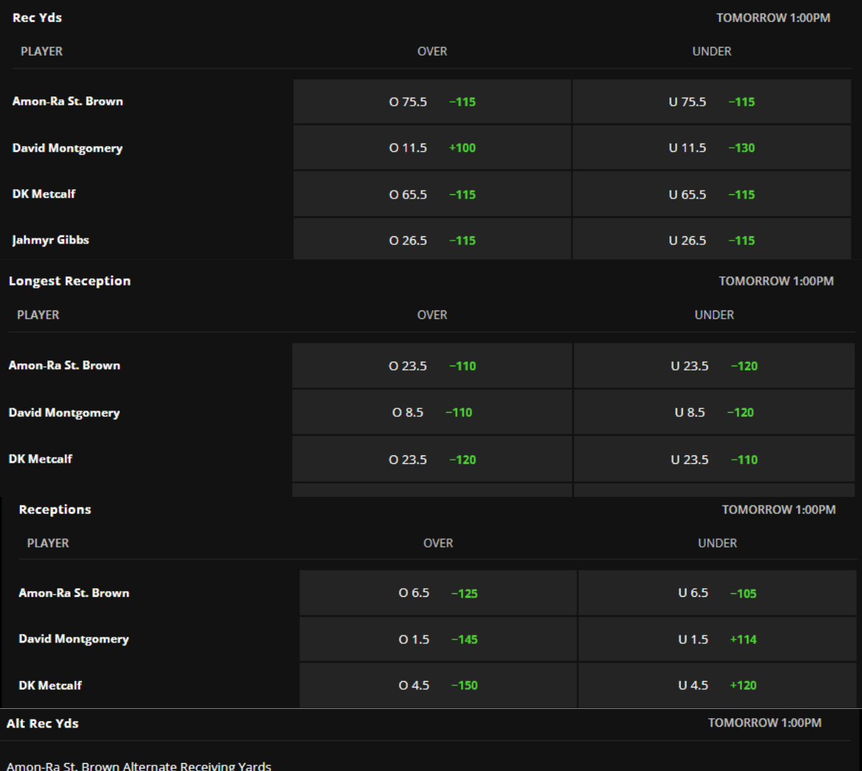
Despite this simple definition, there are numerous derivative markets available for this event type:
These markets are exceptionally prone to inefficiencies as there is far more optionality with each bet. This is in stark contrast to our earlier MLB experiment. Baseball is a fundamentally slower and less variable game, so the derivative options were essentially “yes or no” bets with little room for edge aside from pricing.
However, since these bets offer an “over/under X” approach, we can build out an edge by first predicting a better baseline X value. Furthermore, the bets are offered at an attractive -115 to -130, in contrast to the -250 seen in MLB. To refresh, these odds refer to what you have to pay in order to receive $100 in profit. For example:
-250 means you pay $250 to make $100. 100 bets of 250 for a notional risk of $25,000 will return $10,000, for a return of 40%
-115 means you pay $115 to make $100. 100 bets of 115 for a notional risk of $11,500 will return $10,000, for a return of 87%
So, we definitely want to focus our attention here.
Now, lets build some models.
You Can’t Put A Price Tag on Relationships… Or Can You?
We are attempting to predict a rather difficult real-life problem, so we must first intuitively conceptualize the scenario so that we can choose our initial features.
Since we’re modelling player receptions, we need to quantify the relationship the quarterback has to the players on his team. We first want the model to answer easy questions like:
How often does Quarterback A throw to player B?
What is the maximum distance that Quarterback A usually trusts player B to receive the ball at?
Then, we can answer more complex questions like:
When wind speeds are above 10mph and the temperature is below 60 degrees, who does Quarterback A tend to trust the most?
Under those conditions, do the passes tend to be longer or shorter?
If they tend to be shorter, how much shorter? Are there any outliers?
So naturally, we need data on who the players were, what they did, where they did it, and what conditions were like. Here’s what that looks like before processing:
To capture these complex relationships, we’ll refer to a few old friends.
Our goal is to predict a robust, baseline expected figure, so we will go the route of ensembling, which is where we train and average multiple models to get a single value. To do this, we’ll use tree algorithms and a neural network.
Let’s do a quick refresher on why these will be suitable for our task:
Tree Models
Decision tree models work by creating branches based on our features, here’s an example:
This simple tree attempts to predict the listing price of a house based on the features of square footage and the number of bedrooms and bathrooms. Since we are trying to predict a continuous variable (e.g., length in yards of longest reception), we have to use a regression tree which becomes a bit more involved.
In the above example, this represents just 1 tree. Based on the predictions of the individual branches, it may take an average to represent the prediction, in this case, the average estimate is $250,000. If the true value is $350,000, the model will record that error and use it in the next tree to get closer to the true value. It may apply different weights to the square footage, and different weights to the neighborhood name (e.g., predict higher if the neighborhood has “Lake” or “Meadows” in the name), and so on.
To prevent overfitting, it always splits the data into subsets, optimizes on the initial subset’s errors, then predicts on the next unseen subset, optimizing again, and so on.
XGBoost and Random Forests are currently the de-facto leaders in tree algorithms, so we’ll use them.
Neural Networks
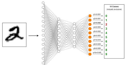
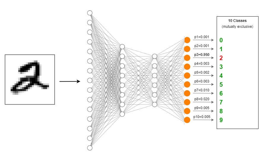
Neural Networks fall under the realm of “black box” algorithms, but they work essentially the same as the prior algorithms. Instead of trees, it uses layers to find optimal weights of the features and takes in the errors of the prior iteration to improve predictions for the next iteration.
It might be a tad bit overkill, but we want to make sure that the predictions of one model don’t vary extremely from each other, so we train all 3 just to be sure.
So, now that we understand the problem and have chosen the appropriate tools, let’s build the solution.


