The Raw Realities of Quantitative Trading
When it's glitzy, it's glamorous. When it's raw, it's raw.
Before we dive in, know that this isn’t a doom-and-gloom post — quite the opposite, actually.
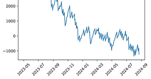
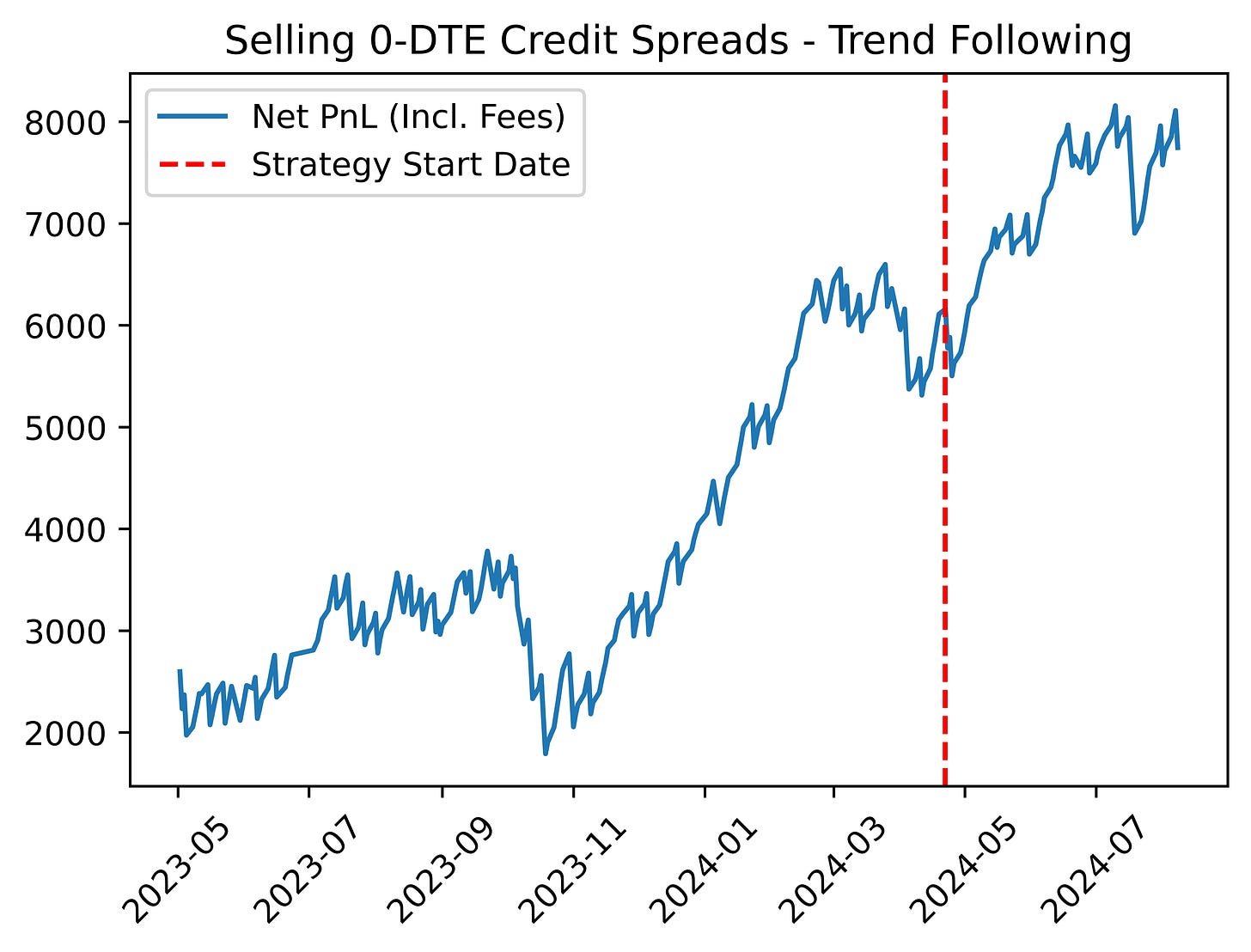
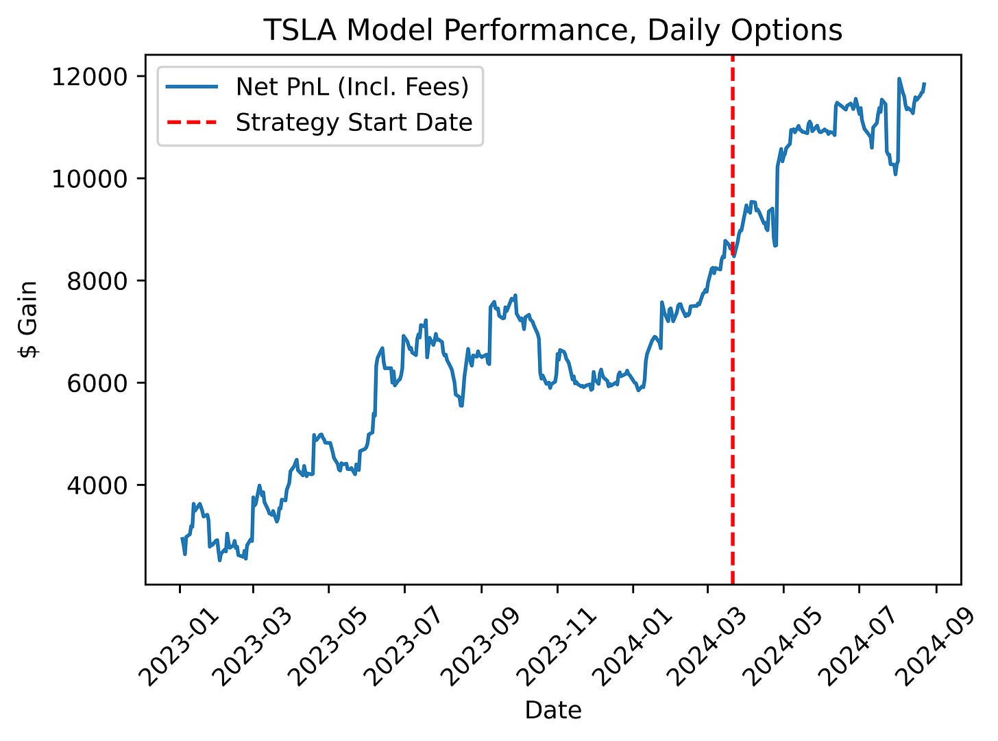
For awhile now, we’ve been running a few systematic strategies in real-time. Most notably, our SPX short volatility strategy and a statistical short term prediction model:
We announced these strategies about 4 months prior to this post and have been letting them run on automated basis, as have quite many of your fellow readers.
Once we were able to see out-of-sample proof that systematic profitability was achievable, it put the batteries in our back to go on and find a whole lot more like it.
In theory, if you have say, 10 of these uncorrelated strategies gunning in tandem, you can allocate a larger chunk of capital and essentially turn into a low volatility, cash-printing enterprise.
There’s been no evidence to the contrary of that, but nevertheless, actually getting there has been a bit more nuanced than first glance. So, today, we’ll be diving deep into the under-mentioned nuances of building a quantitative trading operation from the ground up.
So, without further ado, let’s get right into it.
The Cost of a Really, Really Good Backtesting System
The business model of a trading operation is simple — you form an idea about how a market works, then you use a financial instrument to profit if that idea is correct. Over a long enough time period, you wish for your idea to be correct and pay commensurately more times than it doesn’t.
So, naturally, the first step is to pretend that you had the idea say, a year ago, and see what your performance would have been if you traded on that basis. This being the base-building step is consequently the part that first determines whether the idea lives or dies.
To get a real understanding of how important absolute precision at this step is, let’s go over some real-world examples from our own strategies:
Backtesting SPX
To quickly recap, our SPX strategy uses the VIX1D to help estimate volatility and the range of SPX prices by close. We apply an adjustment to the daily figure and use an SPX trend-following component to determine which direction to sell. In rising bull markets, we sell puts; in falling bear markets, we sell calls — simple.
To backtest this, we first replicated the market environment at exactly 9:35 (5 mins after open when prices have stabilized). We know that in real-trading, we won’t have any information beyond that time, so we make sure our simulation follows the same logic.
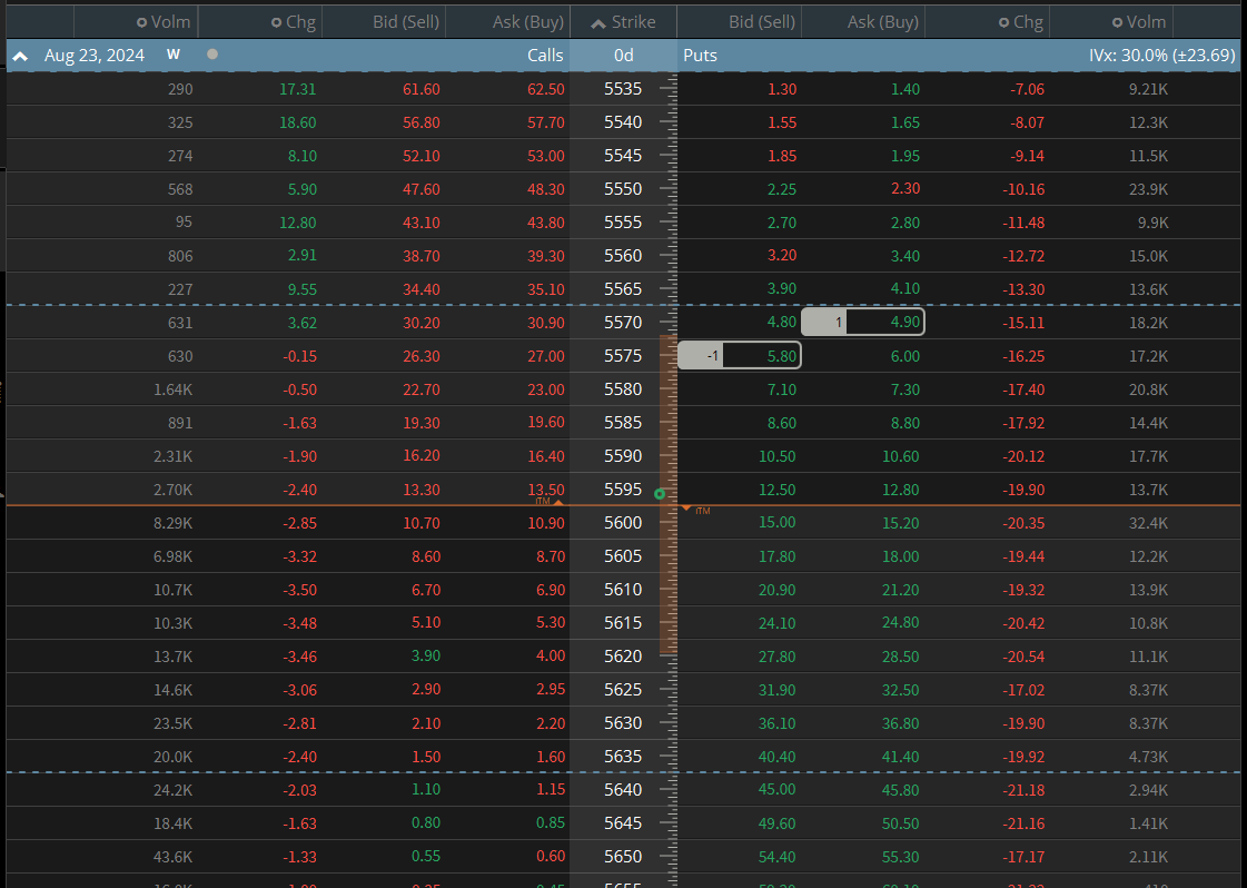
Once we’ve recreated the optimal strikes of the day, we then move onto getting the prices of the credit spread we would sell. To do this, we pulled the closing value of each option in the spread at the respective minute.
For example, if we were to sell the 5000/4995 put spread, we would pull the closing value of the 5000 strike put at 9:36 (we would trade 1 minute after getting the strikes) and the closing value of the 4995 strike put, also at 9:36.
These are 0-DTEs, so if our strikes were correct, the spread should be near worthless at closing time. So, we pull the closing values of the spread at 15:59 (1 minute before close) and save that as the final price of the spread. We calculate our PnL as the price we sold the spread for minus the cost of it at close, before subtracting brokerage/exchange fees.
Now, this is okay enough for a quick, rough, and dirty backtest to test the idea, but there’s a few pretty big mistakes here that we have to fix:
You’ve GOTTA Use NBBO.
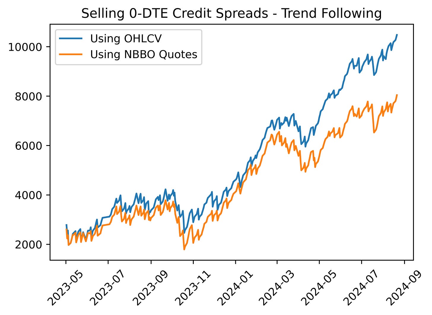
Using open-high-low-close-volume (OHLCV) values when backtesting options is sometimes okay, however, it becomes increasingly unreliable when using deep in-the-money or out-of-the-money options.
A typical 1-minute OHLCV data point typically uses “open” to represent the first trade of that minute and “close” to represent the last trade of that minute. So, even if an option last traded at 9:30:05 but the price of the stock moved 10% by 9:30:30, this endpoint would return the traded price at 9:30:05 which, of course, would not have actually been tradeable.
Further, the last traded price doesn’t always best reflect a price that would have been tradeable due to wide bid/ask spreads and the inclusion of block trades.
Alternatively, we can choose to use quotes of the national best bid and offer (NBBO). NBBO quotes represent the exact listed and tradeable bid/ask quote at the appropriate timestamp. Even for deep ITM/OTM options, the NBBO quotes represent the real prices we would have been able to immediately trade at.
We can use the mid-price of an SPX bid/ask for simplicity (highly liquid/tight), but we can also choose to cross the spread to be more aggressive/realistic.
To see an example of why this distinction is important, let’s examine the simulated performance of our SPX strategy on May 31st, 2024.
On that day, assume we initially sold the spread for 1.20 (average). Using the OHLCV method, let’s pull the value of the spread at the end of the day to calculate our PnL:
Now, let’s use the quotes method:
With using the OHLC endpoint, the PnL of that day appears to be ~-$20, since we sell the spread for 1.20 and buy it back for 1.40. However, using the actual quotes, it appears that the PnL was closer to -$360 since we’d sell the spread for 1.20 and buy it back for 4.80.
In reality, our PnL was much closer to -$360, as SPX closed far above our strike prices, resulting in the max loss (short a call spread on that day).
Now, although this is an outlier example, you’ll see in a moment how even little errors like that can add up.
Contract Specifications Really, Really Matter / Trade Limitations
Our initial PnL method of taking the price we sell the spread for less the price at the end of the day is a close enough approximation, but it’s not exactly what we’d see in the real world.
For starters, routinely selling and buying back the spread in the same day is not allowed unless we have a net liquidating value of >$25,000, so in reality, we would have to hold the contracts until maturity were we to trade everyday like the backtest assumes.
At that point, the EOD value wouldn’t reflect our PnL, but rather the official SPX settlement value:
The official settlement value of SPX at 16:00 (4:00 PM EST) determines the PnL of the spread at expiration.
In the above example, because SPX settled far above the short and long strikes, we took the full max loss of the position for a PnL of ~-$380. This creates yet another observed PnL difference of an extra $20 per contract sold.
So, once we’ve both used the proper method of simulating prices (actual bid/ask) and calculating PnL (proper settlement values), we can have a more realistic and robust backtest:
Although the EV dropped by ~$5 from $22 to $17 when switching to quotes and settlements, the strategy still survived — so, we keep it in production.
In this case, making the backtest more realistic didn’t kill the strategy, but it isn’t always so:
Can you guess which one uses proper quotes and which uses the fast-and-dirty method?
So, making sure that your method of backtesting is actually good and realistic ensures that you don’t have any costly mistakes and that live trading is just as you planned, but it also comes with the “drawback” of killing many strategies before they’re even off the page.
Do a good job of backtesting for long enough, and you’ll have a folder filled with 100-liners that never get opened again — which brings us to another interesting nuance of the job:
Coming Up With Tradeable Alphas
What’s great about our main short option strategy is that it’s as close as we can get to making the markets a giant piggy bank. On any given trading day, once we have the optimal strikes and direction, we can just choose how many contracts to sell, and thus how much the market will pay us, and we’ll receive that amount ~80% of the time.
The problem is that there’s no reward without risk — if we want to make, say, $1,000 a day, we would need to put up ~$4,000 a day as opposed to our current ~$400. This is fine if we had enough capital where we would be able to survive multiple $4,000 drawdowns in a row, which of course is the case for many on the street, but not necessarily for us (yet).
So, when it comes to wanting to make more money, we have 2 options:
Start with more.
Find more uncorrelated strategies that you can allocate to for greater gross profits and lower volatility.
In 99% of cases, option 2 is the more realistic choice.
With us falling in that 99%, let’s take a look at what that process has been like.
To start, we fell in love with the idea of systematic short option strategies — automated trades based on some pre-defined criteria — so we ventured out to test some other strategies just like it:
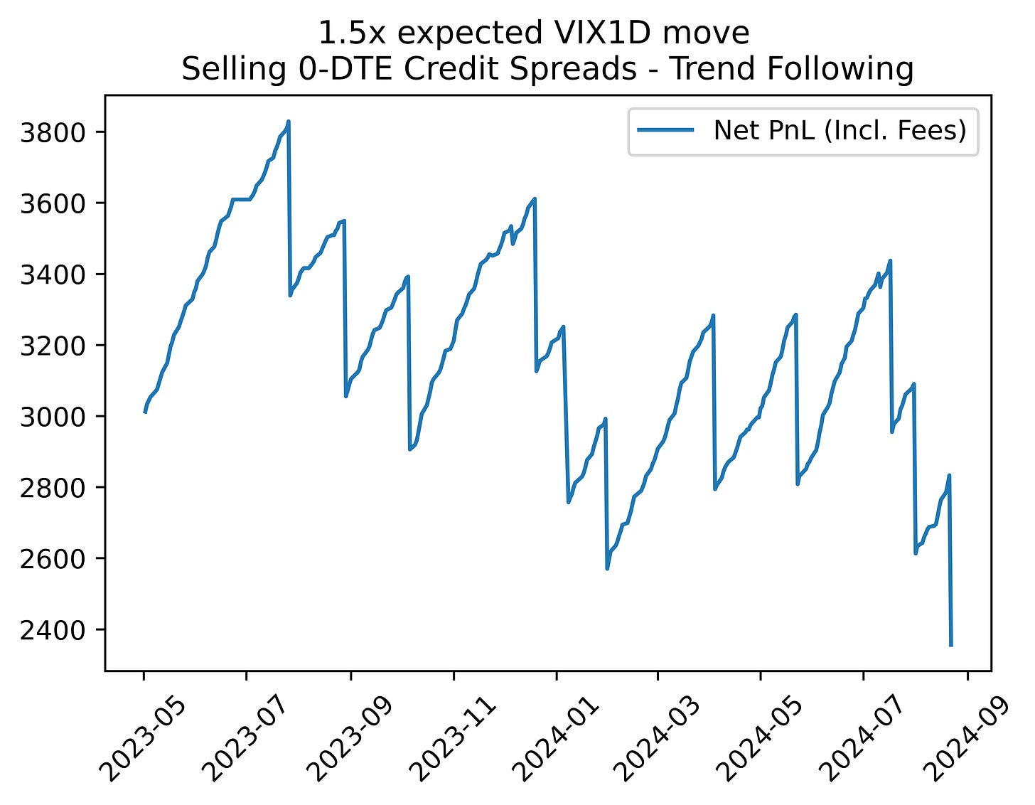
To start, a simple modification of our original strategy. We typically use 0.5x the expected VIX1D move, so let’s try selling just a more conservative multiple of the expected move (1.5x):
You may not be able to tell visually, but this approach had a 95% win rate with an average profit of ~$15 and an average loss of ~$-350 (just 15 recorded losses over 1y).
Unfortunately, because of the extremely negative skew of this approach, it has an expected value of ~$-3. On any given day, there’s a 95% chance you can run this and pull out a few bucks, the challenge just comes from avoiding that 5% where you give it all back.
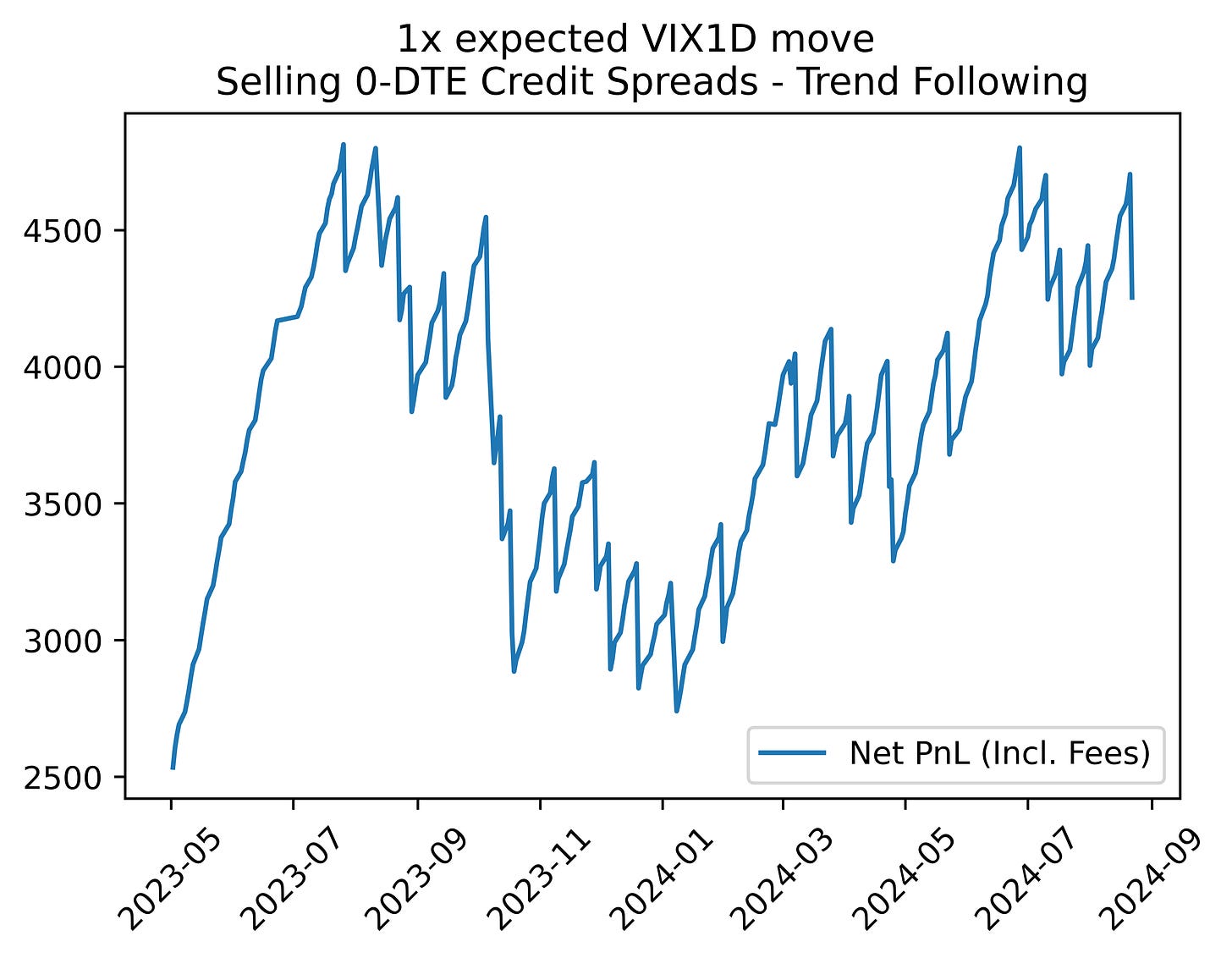
Perhaps we can find a middle ground and just sell the standard expected move (1x)?:
A bit better; this approach had a 91% win rate, for an average profit of ~$45 and an average loss of ~-$400. This version’s EV of $5 is 3x less than our default version, but it represents a potential option.
Realistically however, if we were to add this iteration to our original strategy, we would just be doubling our correlation risk and thus magnifying losses on the bad days while marginally enhancing the good days. At that point, we’d be better off just allocating more to the original strategy — so, this won’t do.
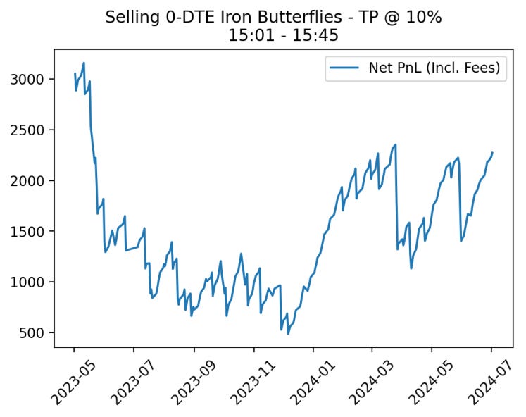
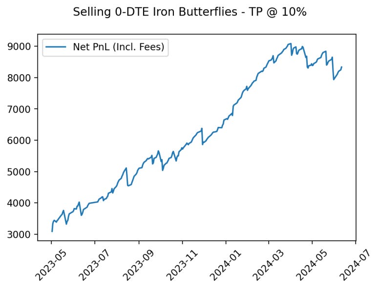
Moving on, we know that there are still millions worth of SPX options that will expire worthless every day, so it’s probably wise to go back to the drawing board of selling those options:
Building on foundational market theories, we know that realized volatility tends to almost always be lower than implied volatility, so perhaps we can move into market neutral bets that are purely based on that relationship.

